Load Planning and Utilization Accounting for 3D-Printed Deliveries

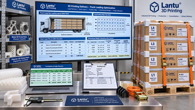
Introduction: Why Per-Unit Freight for the Same Order Can Differ by Nearly Twofold Across Two Shipments

In lantu3D’s delivery practice, the same batch of 300 nylon fixtures, shipped on the same trunk route with the same carrier, incurred freight of CNY 18.6 per part when dispatched as a dedicated shipment. When later consolidated with sample shipments for two other customers and replanned based on volumetric weight, the per-unit freight fell to CNY 10.2. The parts, packaging, and protection level did not change; the only difference was “how much billable space remained in the vehicle.” 3D-printed parts are often low-density, irregularly shaped, and include lattice openings and conformal packaging. Their actual weight may be low while their volume is substantial, so estimating freight based on weight intuition systematically underestimates costs. More troublesome still, once shipments are consolidated, the allocation of charges among three orders, responsibility for signing off on vehicle utilization, and authority over stacking levels often become sources of dispute during month-end reconciliation. This article transforms load planning and utilization from “the shipping operator’s experience” into an auditable calculation sheet. It covers volumetric weight, stacking constraints, multi-order vehicle consolidation, and per-unit freight allocation, serving lifecycle management from design data to physical delivery rather than merely explaining how to load goods onto a truck.

1. First Lock Down the Three Definitions: Actual Weight, Volumetric Weight, and Chargeable Weight

The first step in any load-planning calculation is not vehicle scheduling, but standardizing definitions. Actual weight G is measured on a calibrated scale and includes pallets, reusable containers, cushioning liners, and document pouches, accurate to 0.1 kg. Volume V is calculated from the maximum external length, width, and height of each shipment, multiplied by the non-fillable void factor k, rather than from the bounding box of the part itself. For 3D-printed parts with curved surfaces and lattice structures, k is 1.15–1.35 (1.05–1.10 for regular cartons; use the upper limit for irregular parts after cushioning is added). This factor must be documented in the packaging work instruction and tied to a revision; otherwise, two people can calculate volumes for the same part that differ by 20%. Volumetric weight Wv = V × k ÷ conversion factor. For trunk-road freight, a common convention is 1 m³ ≈ 333 kg (or lane rules such as 6,000 cm³/kg), although the carrier’s current rate card always prevails. Air freight commonly uses 6,000, while express services may use 5,000–8,000; one formula must never be applied indiscriminately to all modes. Chargeable weight Wb = max(G, Wv), and all three values should be printed on the waybill. It is recommended to maintain “lane + conversion factor + rate version + effective date” as four master-data fields that are automatically retrieved before each quotation. Using an old conversion factor on a waybill after a rate-card revision is among the most common and hardest-to-trace errors in consolidated-shipment accounting.

2. Utilization Does Not Mean “Pack It Full”: Three Categories of Constraints Take Priority Over Volume

Vehicle utilization η is defined as the occupied billable volume divided by the vehicle’s effective volume, but constraints must first be deducted from both numerator and denominator. The first category is geometric constraints: the internal vehicle length, width, and height less door frames, wheel arches, and handling clearance (typically 50–100 mm on each side). Effective volume is Veff = (L−2δ)(W−2δ)(H−δtop). The second category is stacking constraints: carton compression strength and fragility-test results determine the maximum number of layers nmax, typically three to five. Cartons containing thin-wall, lattice, or unfinished resin parts must not be placed on the bottom layer, and separators must be placed between layers; separator thickness and weight must also be included in occupied space. The third category is securing and access constraints: straps, anti-slip mats, and dunnage airbags consume 3%–8% of volume, while the rules of heavy items not over light items, large items not over small items, and later deliveries loaded first create non-backfillable voids. Therefore, the practical formula is η = Σ(Vi×ki×ni×ui) ÷ (Veff×(1−r)), where ui is stacking utilization (affected by nmax and load balancing within a layer, typically 0.75–0.92), and r is the securing-space allowance. As a rule of thumb, full-vehicle η ≥ 0.78 qualifies as an acceptable load plan; 0.65–0.78 requires written justification; and 20% across batches, a review must be triggered to determine whether the rate version, k value, or η has changed. Allocation results should be written back to the order cost card alongside material, machine-time, and post-processing costs for the 3D-printed part, enabling quotation reviews.

6. Release Gates and Exception Handling

Establish five D1–D5 release gates before shipment; vehicle sealing is permitted only after all have passed: D1, dimensional and weight data match physical spot checks (sample ≥3 items per shipment, deviation ≤2%); D2, calculated η falls within the target range and the Load Confirmation Sheet is dual-signed; D3, stacking layers, securing photographs, and the heavy-not-over-light check are verified layer by layer; D4, evidence is retained for each of the five consolidation criteria, and declarations plus temperature/humidity requirements are valid; D5, the allocation method is frozen, reconciliation variance is ≤1%, and all three weight fields are complete on the waybill. Exceptions are handled in three states: State A (data-entry or label errors) is corrected and recalculated on site without changing the loading plan; State B (low η, uneven layer loading, or incorrect rate version) requires reloading or reallocation, and vehicle sealing is voided and reapproved; State C (hazardous-goods classification conflict, customer-confidentiality conflict, or an irresolvable out-of-gauge condition) requires removing the entire shipment from consolidation, arranging separate transport, and recording the reason. All A/B/C records are archived by “load-plan number + timestamp + operator + reviewer” and linked with in-transit monitoring and proof-of-delivery records into a single traceability chain. Conduct a quarterly reverse-verification exercise: randomly select a historical waybill and work backward from per-unit freight to the layer number, k value, η, and allocation method. The first-pass rate should be ≥95%.

7. Implementation Checklist and Common Misconceptions

A 30-day implementation can be divided into four weeks: in week one, build master data for effective vehicle volume, conversion factors and rate versions, k-value tables, and nmax-to-Gc mappings; in week two, embed the nine-field load plan and layer diagrams into shipping work orders; in week three, launch allocation calculations and reconciliation-variance checks, running three actual consolidated-shipment batches; in week four, conduct D1–D5 gate audits and reverse-verification exercises. Perform eight self-checks: whether every item uses external dimensions including cushioning; whether actual, volumetric, and chargeable weights are distinguished; whether the k value is tied to the packaging revision; whether stacking levels have test evidence; whether η deducts the securing allowance; whether consolidation passes all five criteria; whether the allocation method is frozen and reconciled; and whether layer numbers and photographs can be traced back from per-unit freight. Five common misconceptions are using the part bounding box as the outer-carton volume, applying one conversion factor to both air freight and trunk transport, treating “filling the vehicle” as a qualified η criterion, considering only direction rather than confidentiality and cleanliness compatibility when consolidating, and allocating freight by impression at month-end. All can be exposed through a single confirmation sheet and one reverse-verification exercise.

Conclusion

The value of load-planning and utilization accounting is not to fill vehicles more completely, but to turn “how much billable space this item occupied, how much freight it should bear, and which layer it was placed on” into signed, auditable, traceable engineering facts. For a full-lifecycle platform such as lantu3D, spanning design through physical delivery, volumetric-weight definitions, stacking constraints, the five consolidation criteria, allocation reconciliation variance, and D1–D5 release gates are all part of the delivery evidence chain, just like process parameters and inspection records. Lock down the definitions, map the layer numbers, and reconcile the variance, and per-unit freight becomes usable data for quotation and process decisions rather than an unexplained month-end expense.