Finite-Capacity Scheduling for 3D Printing Workshops: Engineering Controls from Capacity Load Calculation and Operation-Level Gantt Charts to Material Shortages and Rush Orders

Introduction: Why Is the Shop Still Firefighting After the Schedule Is Complete?

Many additive manufacturing workshops appear to have complete schedules: every machine has orders assigned each day, start times are defined, and promised delivery dates are listed. Yet the shop floor is still firefighting every day—rush jobs jump to the front of the queue, one machine sits idle while another is burdened with six work orders, and promised delivery dates are repeatedly pushed back. The issue is usually not that schedulers are not working hard enough, but that the schedule is built on an assumption of “infinite capacity.” It answers only “which work order should be processed first,” not “after accounting for changeovers, post-processing, inspection, and rework, can this machine actually take on another job?”

Finite Capacity Scheduling (FCS) is an engineering method that upgrades scheduling from a “sequencing list” to a “load plan.” It incorporates the actual occupancy time of every operation, equipment availability calendars, workforce shift structures, fixture and tooling constraints, and material readiness status, then produces a plan that can both be executed and verified.

1. The Difference Between Infinite and Finite Capacity Scheduling

Infinite-capacity scheduling lays an order’s process route across a timeline and checks only the logical sequence between upstream and downstream operations. It does not verify whether a resource is allocated more than once at the same time. The resulting delivery date is often a “theoretical earliest completion date” that is nearly impossible to achieve on an actual shop floor.

Finite-capacity scheduling assigns every operation to a specific resource—equipment, workstation, operator, or tooling—and accumulates the load on that resource within the same time window. When the total exceeds available capacity, the scheduling engine must make a choice: defer the job, switch equipment, outsource the work, or renegotiate the delivery date with sales. This mandatory decision mechanism is exactly what infinite-capacity scheduling lacks.

For 3D printing workshops, this issue is further amplified. The occupancy of a metal LPBF machine includes far more than printing: powder spreading and atmosphere purging, the printing process, depowdering and part removal, support removal, heat treatment, wire EDM, blasting, and inspection. Each stage uses different resources and can vary significantly in duration. Scheduling only the printing operation excludes more than 70% of the actual workload from the model.

2. Building an Operation-Level Time Model: From Experience-Based Estimates to Measurable Data

The foundation of finite-capacity scheduling is operation-level standard time. The following approach is recommended:

1. Printing time. Do not rely on a rough estimate of “number of parts × per-part time.” Actual time = recoating preparation + layer scanning time + build-platform cooling + part removal and depowdering. Scanning time can be estimated from slicing software output, while the other three components should use measured averages by machine type. On a typical four-laser metal machine, non-printing activities usually account for 25%–40% of total machine occupancy per build.

2. Post-processing time. Heat treatment should be scheduled by furnace batch rather than by individual part, because multiple parts can be loaded together but are constrained by furnace volume and process profiles. Wire EDM, blasting, and inspection should be scheduled by part. The key is to establish a “furnace batch capacity” parameter; otherwise, the schedule will treat every part as occupying an entire furnace by itself.

3. Changeover and switching time. Material changes, recoater-blade changes, support-parameter adjustments, and recalibration are all changeovers. In measured practice, a metal machine powder change, including powder sieving, machine cleaning, and atmosphere purging, often requires 2–4 hours; changing a material spool on a polymer machine typically takes 30–60 minutes. Without modeling changeovers, scheduling will systematically underestimate the load.

4. Probabilistic time for rework and scrap. Add expected rework time to each operation based on historical yield. For example, with a 95% build yield, expected rework time = per-part processing time × 5%. This is not a pessimistic estimate; it simply incorporates known statistical facts into the plan.

3. Capacity Load Calculation: Determine Whether More Work Can Fit Before Scheduling

Once operation times are available, load calculations can be performed. The core formulas are straightforward:

Operation load (hours) = Σ (standard operation time for each work order + changeover time + expected rework time)

Available resource capacity (hours) = calendar hours × availability rate × shift factor

Load rate = operation load ÷ available resource capacity

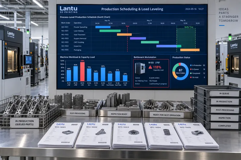
A practical engineering guideline is as follows: a load rate above 100% requires deferral or load redistribution; a sustained load rate between 85% and 95% indicates that the resource is a bottleneck with no buffer, meaning any disruption will directly become a delay; a load rate below 60% calls for a review of whether scheduling rules are overly conservative or the order mix is unbalanced.

Availability rates should not be guessed. Use actual data from the previous three months: available operating hours ÷ calendar hours, after deducting planned maintenance, unplanned downtime, waiting for materials, and waiting for inspection. Many workshops believe their availability rate is 90%, while measurement shows only 72%—a single parameter that can explain much of the delivery-date variance.

4. Operation-Level Gantt Charts and Buffer Management

The output of finite-capacity scheduling should be an operation-level Gantt chart: time on the horizontal axis, resources such as equipment, workstations, and personnel on each row, and each colored block representing one operation. The length of each block should equal the calculated processing time, not an “ideal duration.” This makes bottlenecks immediately visible—the resource with uninterrupted blocks and downstream operations constantly waiting is the constraint that should be addressed first.

Buffers must be established on top of the Gantt chart. A two-tier buffer system is recommended: a delivery buffer at the end of the order to absorb the impact of process variability on the committed date, and a bottleneck buffer before the bottleneck operation to ensure the bottleneck never runs short of work. Buffer consumption is one of the most effective early-warning indicators. When more than 50% of the delivery buffer has been consumed while physical progress is below 40%, the order should be marked as at risk and the customer should be proactively informed, rather than waiting until three days before shipment.

5. Material Shortages and Rush Orders: The Two Most Common Sources of Schedule Distortion

Material shortages. A schedule may assume that all materials are ready, but an uninspected powder batch, an unavailable build plate, or a queue at an outsourced heat-treatment provider can prevent a “ready-to-start” work order from actually starting. The solution is to add a material-readiness prerequisite check to every work order: the powder batch has an inspection report, the build plate is in stock, tooling is available, and the outsourcing time slot is confirmed. Only when all four conditions are met may the order enter the schedulable pool. The shortage list should be updated daily on a rolling basis rather than discovered on the scheduled start date.

Rush orders. Moving a rush job to the front is essentially a local optimization that bypasses scheduling rules. The correct approach is not to prohibit rush orders, but to assign them a cost: their impact on the delivery dates of work orders already in process must be explicitly assessed, including how many orders are affected and how many days each will be delayed, and the rush order must explicitly consume bottleneck buffer. The scheduling engine should provide a “before-and-after rush-order comparison,” allowing decision-makers to choose with full knowledge of the cost rather than letting the shop floor compete for equipment based on intuition.

A schedule freeze period should also be defined. For example, the sequence of work orders scheduled to start within the next 48 hours can be frozen, with any changes during that period requiring approval. Without a freeze period, the schedule will always be disrupted as soon as it is completed, and load calculations will lose their meaning.

6. Closing the Loop with Metrics: OTD, Schedule Attainment, and Scheduling Variance

Completing a schedule does not mean management is complete. The following three metrics should be tracked and reviewed weekly:

1. On-time delivery (OTD). Measure against committed order dates, distinguish between customer-caused and internal causes, and assess only delays caused by internal factors.

2. Schedule attainment. Actual completed operations ÷ planned completed operations, reported by resource group. This metric directly indicates whether the time model is accurate.

3. Scheduling variance. The distribution of variance between actual and standard time. If an operation consistently shows positive variance exceeding 20%, standard time should be revised rather than continuing to pressure the shop floor.

The three metrics must be reviewed together. Poor OTD with high schedule attainment indicates that the time model is too optimistic or promised lead times are too tight. Low schedule attainment with acceptable OTD indicates that the shop is relying on overtime and rush-order interventions to hold performance together, while risk continues to accumulate.

Conclusion

Finite-capacity scheduling is not an initiative that delivers results simply by purchasing software. In essence, it requires a workshop to translate “experience” into “parameters”: operation-level processing times, equipment availability rates, changeover times, furnace-batch capacity, material-readiness prerequisites, and buffer strategies. These parameters will inevitably be inaccurate at first, but with schedule attainment and scheduling variance as feedback, they can converge to usable accuracy within three months.

For a full-lifecycle management platform such as lantu3D, covering everything from blueprint design to physical delivery, the value of a schedule lies not in how fully it is packed, but in whether it can be verified, made accountable, and continuously improved. Transforming a schedule from a sequencing list into an engineering document with load, buffers, and variance feedback is how delivery dates become not merely a “promise,” but a calculable result.