Melt Pool Stability and Process Window Calibration in Laser Powder Bed Fusion: An Engineering Approach from Keyholing and Lack of Fusion to Releasable Parameters

Introduction: Parameters That Have Been "Tuned In" Do Not Equal a Stable Process

In metal laser powder bed fusion (LPBF) operations, the most common frustration is not "we cannot build it," but rather "it worked this time, but not the next time." On the same machine, with the same batch of powder, parameters that worked last month may produce widespread lack of fusion this month; after replacing the protective window, surface quality may suddenly deteriorate; with a different placement location, the same parameter set may produce keyhole pores in thin walls. The root cause of such fluctuations is often not that the parameters themselves are wrong, but that the team has never managed them within a measurable, reproducible, and releasable process window.

A process window refers to the range of combinations among four variables—laser power, scan speed, hatch spacing, and layer thickness—that, under given material, machine-condition, and geometric constraints, can stably produce dense tracks without triggering defect mechanisms. The purpose of calibration is not to find "one good parameter set," but to map the boundaries and understand how much margin exists between the current production parameters and those boundaries.

1. Three Melt Pool Failure Modes: Keyholing, Lack of Fusion, and Spatter

There are only three typical melt pool failure modes, corresponding respectively to excessive energy input, insufficient energy input, and disturbance.

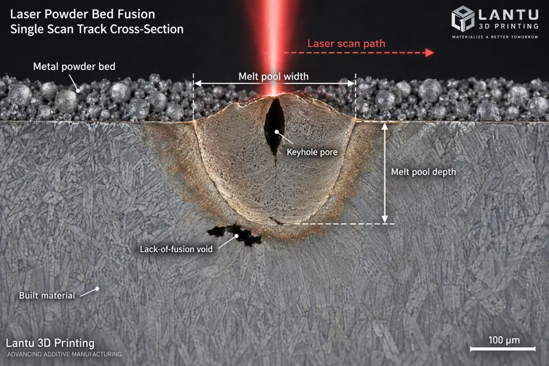
Lack of Fusion: When energy is insufficient or hatch spacing is too large, a melt track cannot effectively overlap with adjacent tracks or the previous layer, leaving irregular pores that are flat, sharp-edged, and often contain unmelted powder. A typical cause is loss of control over the ratio between layer thickness and melt depth—when melt depth is less than 1.5 times the layer thickness, lack-of-fusion defects are very likely to remain at interlayer bonding interfaces. Such defects are distributed in layers along the powder spreading direction and are preferential initiation sites for fatigue cracks.

Keyhole: Excessive energy density causes intense metal vaporization, and vapor recoil pressure presses a deep, narrow depression into the melt pool. After this depression becomes unstable and collapses, vapor and shielding gas are entrapped in the solidification front, forming spherical pores with smooth inner walls. These pores are often located at the bottom of the melt pool and appear in chains along the scan direction. Keyholing is reversible: reducing power or increasing scan speed can move the process out of it. However, its onset is abrupt; once the threshold is crossed, the number of pores does not increase linearly but rises in a step change.

Spatter: The vapor plume above the melt pool ejects molten droplets, typically 50–200 μm in size. Some spatter lands on the powder bed and forms large-particle inclusions, while some lands on the protective window, causing local absorption and heating, which further changes the actual energy reaching the powder surface. This is a typical positive-feedback degradation chain and the physical source of the phenomenon where builds become progressively worse.

2. Do Not Rely Only on Volumetric Energy Density: Normalized Enthalpy Predicts Keyholing Better

The industry commonly uses volumetric energy density E = P / (v × h × t), in J/mm³, to compare parameters. It is convenient for communication, but it has a fatal flaw: it implicitly assumes that melt pool dimensions scale linearly with parameters, while the actual melt pool results from coupled heat conduction and phase transformation. At the same E value, a high-power/high-speed combination and a low-power/low-speed combination can produce completely different melt pool morphologies—one stable and the other already in the keyhole regime.

A more reliable criterion is normalized enthalpy ΔH/hs, the ratio between melt pool input enthalpy and the material’s enthalpy of melting, which incorporates material absorptivity, thermal diffusivity, melting point, and superheat. In engineering practice, a simplified form can be used for judgment: once normalized enthalpy enters a certain threshold range, the melt pool width-to-depth ratio (width/depth) rapidly drops from the conduction-mode range of 1.2–1.8 to below 1.0, entering keyhole mode. Using melt pool width-to-depth ratio as a measurable shop-floor proxy indicator is far more effective than staring at energy density numbers: after single-track samples are mounted and polished, melt width and melt depth can be measured directly under a metallographic microscope, with low cost and an intuitive criterion.

3. Process Window Calibration: A Three-Stage Progression from Single Tracks to Bulk Specimens

It is recommended to divide calibration into three stages and converge gradually, avoiding the immediate fabrication of large numbers of test specimens.

Stage 1: Single Track. Scan single tracks on a substrate using a power × speed grid, with sufficiently large spacing to avoid interaction between adjacent tracks. Observe track continuity: regions with obvious balling or discontinuity should be eliminated directly; regions with continuous tracks, straight edges, and width-to-depth ratios of 1.2–1.8 enter the candidate zone. This step requires only one substrate and has the lowest cost, yet it can eliminate about half of the parameter space.

Stage 2: Bulk Density Matrix. Within the candidate zone, select a 3×3 or 4×4 power–speed combination matrix and print 10 × 10 × 10 mm cubic specimens. Measure relative density using the Archimedes method and combine it with metallographic cross-section porosity statistics. In engineering practice, relative density ≥ 99.5%, metallographic porosity < 0.5%, and no chains of spherical pores are used as the criterion for the dense region. The highest density point is often close to the keyhole boundary, so do not select the density peak as the production parameter. Instead, select the center of the dense region so that there is margin to both the lack-of-fusion boundary and the keyhole boundary.

Stage 3: Geometric Sensitivity Verification. Re-test using feature coupons containing thin walls (0.3–0.5 mm), overhangs, sharp corners, and small holes. Thin walls have poor heat dissipation and severe heat accumulation, and in actual production they often expose keyholing earlier than bulk specimens. This step determines the geometric applicability range of the process window, and the work instructions must state clearly that "this window applies to structures with wall thickness ≥ X mm."

4. Defocus and Spot Size: The Overlooked Fourth and Fifth Variables

Many teams perform very detailed calibration but fail to include defocus and spot diameter in control. Taking a common Gaussian spot as an example, the nominal focal spot is about 70–80 μm. For every 0.5 mm shift in defocus, the spot diameter reaching the powder surface can expand from 80 μm to more than 120 μm, and the power density drops by about half—enough to push parameters from the middle of the window into the lack-of-fusion region. Therefore, defocus must be controlled at the same level as process parameters: after every protective window replacement, optical path adjustment, or galvanometer replacement, focus calibration should be performed again and the measured spot size recorded, rather than continuing to use factory values.

Also underestimated is the actual attenuation of laser power. Calibration uses nominal power, while the power reaching the powder surface is affected by window contamination, fiber aging, and cooling-water temperature. Practical maintenance experience shows that a measured power deviation greater than 5% should trigger window re-calibration, and the measured power rather than the nominal power should be written into the parameter sheet. This requirement should be tied to the optical system maintenance checklist cycle—galvanometer zero position, protective window transmittance, and power calibration—in the same work instruction.

5. Spatter and Gas Flow: Turning Observation into Quantitative Indicators

Spatter is often treated as a minor problem of the shop floor being "a little dirty," but in fact it is a leading signal of the energy state. There are three feasible quantification methods: first, place sampling plates above the powder bed to count the number of spatter particles per unit area and their size distribution; second, use coaxial or off-axis cameras to record plume morphology and brightness fluctuations; third, periodically measure the transmittance decay rate of the protective window. None of these three requires expensive equipment, yet they can turn "it looks about the same" into time-series data.

Shielding gas flow also needs to be quantified. If cross-flow velocity is too low, plume and spatter create shielding and scattering along the laser path, causing energy attenuation and instability; if it is too high, it may disturb fine powder and damage powder bed uniformity. A common engineering range is 2–4 m/s, with the flow field required to remain uniform across the working area. Nonuniform gas flow has a very recognizable signature: forming quality varies systematically with position in different regions of the powder bed, rather than fluctuating randomly. When such "position-dependent defects" occur, the first suspect should be gas flow or powder spreading, not the parameters.

6. Turning the Process Window into Executable Release Rules

The value of calibration is realized only after it is written into rules. A usable process window document should include at minimum: applicable material and batch, machine number and measured power, measured spot size and defocus, the four key parameter elements and allowable fluctuation bands, dense-region boundaries and margin explanation for the selected working point, geometric applicability range, re-calibration trigger conditions (window replacement, powder batch change, power deviation > 5%, machine downtime exceeding the specified duration), and first-article confirmation method.

For the release stage, it is recommended to bind a standard coupon to the process: print one density/feature specimen with each batch or shift in the same build. If its density fails to meet the requirement, the process state of that batch should be judged abnormal, rather than waiting until finished-product inspection to discover the problem. In this way, the process window changes from "engineering knowledge" into "production-line rules," and the quality-control gate is moved forward from final inspection to the process itself.

Conclusion

LPBF process stability does not come from experience-based fine tuning, but from mapping boundaries, quantifying margins, and writing them into rules. Remember three actions: use melt pool width-to-depth ratio and normalized enthalpy instead of single energy density to judge keyholing; use the three-stage progression of single tracks, bulk specimens, and feature coupons to converge the window while retaining margins in both directions; and bring defocus, spot size, measured power, spatter, and gas flow under the same level of control as the parameters. By doing these three things, the problem of "it worked this time, but not the next time" will be greatly reduced, and process capability will truly become deliverable, reusable, and auditable.