Statistical Process Control (SPC) for Volume 3D Printing Delivery: An Engineering Approach from Key Characteristics to Closed-Loop Out-of-Control Response

Introduction: Why Quality Control for 3D Printing Cannot Rely Solely on Final-Part Inspection

As metal and polymer additive manufacturing moves toward low-volume and volume delivery, many teams still use a familiar quality-inspection approach: after each build and post-processing cycle, they sample finished parts for dimensional, visual, and mechanical inspection; conforming parts are released, while nonconforming parts are reworked or scrapped. This approach may remain manageable at production levels of dozens of parts per month. However, once operations reach hundreds of parts per week, with multiple machines running in parallel and multiple powder lots in use, three structural problems emerge.

First, inspection results arrive too late. When final-part inspection detects a shift, dozens of products may already share the same deviation, making traceability and sorting far more costly than in-process containment. Second, the decision criteria are too coarse. A binary pass/fail judgment conceals process-drift trends. A gradually deteriorating process can remain within tolerance for multiple consecutive batches before it suddenly exceeds the limit. Third, assigning responsibility becomes difficult. Without process data archived by batch, machine, and powder lot, teams can only rely on experience-based assumptions and cannot establish a reusable process-improvement loop.

The value of statistical process control (SPC) lies in moving quality control from final-stage judgment to in-process monitoring. It does not replace first-article qualification or final-part inspection; rather, it establishes a continuous, quantifiable band of process stability between them, allowing shifts to be identified before they become nonconforming products.

1. The Prerequisite for SPC: Determine What to Monitor First

The most common reason for unsuccessful SPC implementation is selecting the wrong monitoring targets. An additively manufactured part may have dozens of dimensional characteristics. If all of them are included in control charts, the cost of data maintenance will quickly exceed the benefits. A practical approach is to begin with Key Characteristics (KCs) and apply a tiered screening process.

Key characteristics are typically identified through three perspectives. The first is functional: dimensions involved in assembly fit, sealing, load bearing, or motion, such as the diameter of a mating hole, the flatness of a locating surface, or the depth of a sealing groove. The second is process-related: characteristics with the greatest historical variation on the same machine, such as wall thickness in thin-wall parts, flatness of large surfaces, or angular deviation on overhang surfaces. The third is failure-related: characteristics repeatedly identified in past customer complaints, rework records, and scrap records.

After cross-screening these three perspectives, a typical part will usually retain only three to eight key characteristics. Each KC should be clearly identified on the drawing or inspection sheet, along with its measurement method, gauge resolution, and sampling frequency. One frequently overlooked constraint is that control-chart resolution depends on gauge resolution. If a gauge has a resolution of 0.01 mm while the process standard deviation of the measured characteristic is only 0.003 mm, the chart will show obvious stepwise stratification and its ability to detect unusual variation will be substantially reduced. Gauge resolution should generally be no greater than one-tenth of process variation.

2. Control-Chart Selection and Out-of-Control Rules

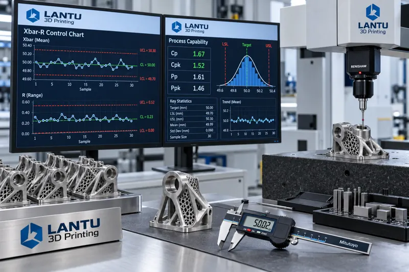
For variable-type key characteristics, the most commonly used chart is the Xbar-R chart. At each sampling point, three to five parts are selected to form a subgroup, and the subgroup mean and range are calculated and plotted on separate charts. The mean chart monitors whether the process center has shifted, while the range chart monitors whether process variation has increased. Both charts should be interpreted together: if the range chart is out of control while the mean chart remains in control, variation has increased but the center has not shifted. Common causes include a change in powder lot, fluctuations in machine condition, or reduced operator consistency. If the mean chart is out of control while the range chart remains in control, a systematic shift has occurred. Common causes include recoater wear, contamination of the optical system, or drift in build-plate leveling.

Control limits should be calculated from actual process data. Typically, at least 25 consecutive subgroups of stable data are used, and the upper and lower control limits are determined from the average subgroup mean plus or minus three estimated standard deviations. It is important to emphasize that control limits and tolerance limits are entirely different concepts. Control limits describe what the process can actually achieve, whereas tolerance limits describe what the customer requires. The process capability index, Cpk, is the bridge between the two because it considers both centering error and dispersion. A commonly used industry threshold is Cpk of at least 1.33, corresponding to a theoretical proportion of approximately 99.99% within the tolerance band. For safety-related or high-value characteristics, the requirement may increase to 1.67 or higher.

In addition to the basic rule of a single point beyond a control limit, internationally recognized out-of-control criteria include nine consecutive points on the same side of the centerline, six consecutive increasing or decreasing points, 14 consecutive alternating up-and-down points, and two out of three consecutive points beyond two standard deviations on the same side of the centerline. These rules identify patterns with very low statistical probability and are intended to capture nonrandom process changes before a limit is crossed. In additive manufacturing, six consecutive increasing points often indicate progressive process degradation, such as a gradual reduction in protective-window transmittance; nine points on the same side of the centerline often indicate a change in process parameters or material lot.

3. Practical Implementation of Sampling Design and Data Collection

Sampling design determines both control-chart sensitivity and maintenance cost. Samples within a subgroup should be produced on the same machine, from the same batch, and within a similar time period whenever possible, so that within-subgroup variation reflects short-term random variation. Between subgroups, sampling should span potential sources of variation such as shifts, powder lots, and machine-maintenance cycles, allowing between-subgroup variation to reveal special causes. This sampling principle corresponds directly to SPC theory: within-subgroup variation estimates random error, while differences between subgroups estimate traceable causes.

The data-collection stage is often underestimated. Manual transcription followed by spreadsheet entry may be feasible for low-volume production, but data delays and transcription errors significantly weaken the real-time value of control charts. A more robust approach is to connect measurements of key characteristics directly to data-acquisition terminals. Results from coordinate measuring machines, vision measuring systems, laser scanning, and industrial CT should be automatically stored in a structured database and indexed by part number, batch number, machine number, and powder-lot number. When a control chart signals an out-of-control condition, the system can directly retrieve process-parameter records, environmental records, and machine-status records from the relevant time window, linking the signal to potential causes.

For teams that do not yet have automated collection capabilities, a practical compromise is to begin with SPC on the highest-value production line and three key characteristics, using standardized inspection sheets and daily summary forms for manual maintenance. After validating the method, it can be expanded gradually. Treating SPC as a one-time, enterprise-wide rollout often leads to abandonment within a few months because the data-maintenance burden becomes excessive.

4. Response Procedures After an Out-of-Control Signal

An out-of-control signal from a control chart is only the beginning; the response procedure is what ultimately determines SPC effectiveness. A complete response loop typically includes four steps. The first is confirmation of signal validity, excluding gauge abnormalities, data-entry errors, and sample-identification errors. The second is scope definition: determine the affected batches, machines, and time window. When necessary, trace backward to the last in-control point and lock forward through the point at which corrective action became effective. The third is root-cause investigation, checking each of the six dimensions of people, machine, material, method, environment, and measurement, with priority given to the most recent changes before the signal occurred. The fourth is action and verification: after corrective action is taken, collect at least five new subgroups to confirm that the process has returned to statistical control and update the process capability index.

All out-of-control events, root-cause analyses, corrective actions, and verification results should be archived as searchable records. Their value lies in building an internal failure-mode library: when a similar signal recurs, investigation time can be reduced from hours to tens of minutes. This is also the interface between SPC and a knowledge-management system. Process data itself is neutral; only when combined with historical cases does it become engineering capability.

5. Common Pitfalls and Implementation Recommendations

The first common mistake is setting control limits equal to tolerance limits. This delays detection until nonconforming product has already been produced, eliminating SPC's early-warning value. The second is failing to update control limits over an extended period. After process improvements, machine replacements, or changes in material systems, process capability may have changed. Old control limits may be either too loose to remain sensitive or too strict, generating excessive false alarms. Control limits should be recalculated at least every six months or after any major process change. The third mistake is monitoring without improvement. If control charts run stably but Cpk remains around 1.0 for a prolonged period, the process is controlled but lacks sufficient capability. At that point, the focus should shift to systematic process optimization rather than tighter inspection.

For teams beginning SPC implementation, the recommended sequence is: select one production line and three key characteristics; complete gauge-resolution verification and measurement-system analysis; collect more than 25 subgroups to establish initial control limits; implement out-of-control rules and response procedures; evaluate false-alarm rates and containment effectiveness after two months of operation; then decide whether to expand. The overall cycle typically requires three to four months, with investment concentrated in measurement and data rather than in software tools themselves.

Conclusion

Statistical process control provides an engineering framework for volume 3D printing delivery, from key-characteristic identification and control-chart signal detection to a closed-loop response process. It does not alter the process itself, but it makes process conditions observable, quantifiable, and predictable. For additive manufacturing companies, the real challenge of SPC is not statistical theory, but rather the reliability of the measurement system, the continuity of data collection, and whether a rigorously executed response procedure exists after an out-of-control signal. When these three elements are firmly established, quality control can shift from sorting nonconforming products to preventing them, improving both delivery consistency and cost structure in volume production.