Design of Experiments for 3D Printing Process Development: An Engineering Path from Orthogonal Screening and Response Surface Modeling to Process Window Qualification

Introduction: Why Parameter Optimization Keeps Going in Circles

In on-site tuning of metal laser powder bed fusion (LPBF) and polymer sintering processes, a common scenario is this: an engineer increases laser power from 250 W to 280 W, density rises by 0.3%, and the power is increased further. At 300 W, keyholing appears, so the engineer adjusts it downward again. After more than a dozen test coupons, the result is a fragmented empirical curve that must be rebuilt when changing machines or powder batches. The issue is not a lack of engineering effort; rather, the one-factor-at-a-time approach cannot address interactions. Power and scan speed jointly determine volumetric energy density, while powder layer thickness changes melt-pool heat dissipation. These three factors are coupled, and changing one variable at a time can never reveal the full picture.

Design of Experiments (DoE) provides an engineering pathway for solving such multi-factor coupling problems: estimating factor main effects, interaction effects, and response surfaces with the fewest possible test coupons, while defining releasable process windows with confidence intervals. For 3D printing process development, this article presents a complete, practical method from orthogonal screening and response surface modeling to window validation.

1. Distinguish the Three Types of Experiments: Screening, Modeling, and Validation

Process development cannot be completed in a single experiment. It generally proceeds through three levels, each with different objectives, numbers of factors, and sample requirements.

The first level is screening experiments, intended to identify the truly significant 2–4 factors from 6–10 candidate factors. Typical candidates include laser power, scan speed, hatch spacing, layer thickness, preheat temperature, scan strategy (stripe width), interlayer rotation angle, and shielding-gas flow rate. Partial factorial or Plackett-Burman designs can complete screening in 8–12 runs, using density and surface roughness as two broad response metrics.

The second level is modeling experiments, intended to establish a response surface model for the 2–3 key factors identified during screening. Central composite designs (CCD) or Box-Behnken designs are commonly used. A three-factor CCD includes 6 axial points, 8 cube points, and 6 center-point replicates, for a total of 20 runs. Responses are expanded to include density, tensile strength, dimensional deviation, and surface roughness Ra.

The third level is validation experiments. Print 3–5 confirmation points repeatedly within the model-predicted optimum region and verify that the deviation between predicted and measured values remains within ±5%. Once validation is passed, tighten the window boundaries by 10% to define the parameter range for the production process card.

2. Orthogonal Experiments: Covering the Largest Space with the Fewest Coupons

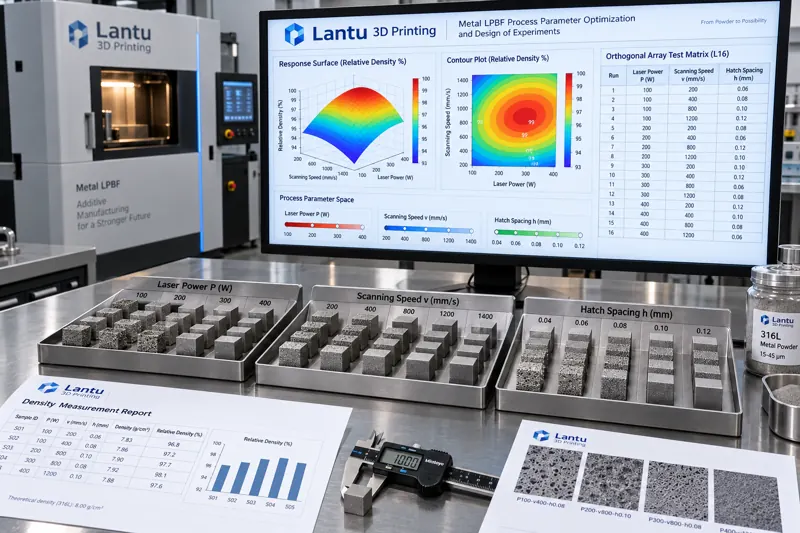
When the number of factors is limited and each factor has the same number of levels, orthogonal arrays are the most economical choice. For 316L stainless steel LPBF, consider three factors at three levels: laser power P, scan speed v, and hatch spacing h. A full factorial design requires 27 runs, whereas an L9(3^4) orthogonal array requires only 9.

For a specific design, set P at 200/240/280 W, v at 800/1000/1200 mm/s, and h at 0.09/0.11/0.13 mm. Following the L9 arrangement, print one set of 10 × 10 × 10 mm cubic specimens for each level combination. Measure density using the Archimedes method and record surface roughness Ra.

Range analysis can quickly rank factors: calculate the mean response at each level for every factor, with range R = max(mean response) − min(mean response). A larger R indicates a more significant factor effect. If R(P) = 2.1%, R(v) = 1.4%, and R(h) = 0.6%, the order of importance is power > speed > hatch spacing. Further analysis of variance (ANOVA) uses the F-test to determine significance: factors with F values above the critical value and p values below 0.05 proceed to the next modeling stage.

The limitation of orthogonal experiments is that they assume no interactions between factors. If strong coupling between power and speed is suspected—because volumetric energy density E = P/(v·h·t) is inherently a multiplicative relationship—response surface design should be used during the modeling stage rather than forcing continued use of an orthogonal array.

3. Response Surface Methodology: From Discrete Points to Continuous Surfaces

The core of response surface methodology (RSM) is fitting the relationship between responses and factors with a quadratic polynomial:

Y = β0 + Σβi·xi + Σβii·xi² + Σβij·xi·xj + ε

Here, the cross term βij is the quantitative expression of an interaction effect. For a CCD, the key parameter in a three-factor design is the axial distance α. For a rotatable design, α = 2^(k/4) = 2^(3/4) ≈ 1.682, where k is the number of factors. Axial points are located at ±1.682 in coded space, cube points at ±1, and center points are repeated six times to estimate pure error.

Three checks are essential after fitting. First, the lack-of-fit test: a p value greater than 0.05 indicates no significant discrepancy between the model form and the data. Second, the coefficient of determination R² and adjusted R²: the difference between them should be less than 0.2, otherwise overfitting may be present. Third, residual normality and homoscedasticity must be checked. In practice, R² may reach 0.95 while adjusted R² is only 0.86; in this case, non-significant higher-order terms should be removed before refitting.

Multi-response optimization is challenging in 3D printing: density should be maximized, roughness minimized, and dimensional deviation brought close to zero, yet these objectives often conflict. In engineering practice, a desirability function maps each response to a 0–1 scale, after which their geometric mean is used to obtain an overall desirability D. The parameter combination at the maximum D is selected. Weights are assigned according to customer acceptance priorities; for example, aerospace components may use weights of 0.5 for density, 0.3 for roughness, and 0.2 for dimensional deviation.

4. Process Window Qualification: Turning an Optimum Point into a Releasable Range

Finding the optimum point is only the first step; production requires a range. A practical approach is the overlay contour plot: plot the acceptance threshold for each response as a contour line—density ≥ 99.5%, Ra ≤ 12 μm, and dimensional deviation ≤ ±0.1 mm—and use the overlapping area of all contours as the process window.

Once the window is established, a safety margin must be retained. A recommended practice is to shrink the window boundary inward by 10%. For example, if the model gives a feasible power range of 235–265 W, the process card should specify 238–262 W. Powder-batch variation, drift in shielding-gas purity, and optical-system power degradation can all gradually shift the actual process point. Maintaining a margin can increase the process capability index Cpk from 1.0 to above 1.33.

Window validation should use three confirmation batches, each containing five parts. For each batch, print one set at the window center, one just inside the upper boundary, and one just inside the lower boundary. If all three consecutive batches pass and inter-batch mean drift is less than one-third of the response standard deviation, the window can be considered stable. Validation data should also be entered into the process record as a baseline for future traceability.

5. Common Pitfalls and Checklist

Pitfall 1: treating the number of test coupons as the entire cost. In fact, 9 orthogonal runs plus 20 CCD runs cost far less than 30 blind one-factor-at-a-time iterations, while producing a reusable model.

Pitfall 2: ignoring block effects. If 20 CCD runs are completed over three days, changes in machine condition, powder batch, and ambient temperature and humidity can be mixed into the residual error. The correct approach is to include date as a blocking factor in the design, or arrange center-point replicates within each block to monitor drift.

Pitfall 3: looking only at density. A process point that achieves 99.5% density may not meet mechanical-property requirements, because lack-of-fusion defects can be underestimated by density measurement. At a minimum, tensile strength and elongation should be tested concurrently; metallographic examination and industrial CT spot checks should be added where necessary.

Execution checklist: Do factor levels cover the range in which the machine can operate stably? Are center-point replicates included to estimate pure error? Has a lack-of-fit test been performed? Do multi-response weights align with customer acceptance criteria? Does the window retain a 10% margin? Do validation batches cover the window boundaries?

Conclusion

Design of Experiments transforms 3D printing process development from empirical trial and error into a measurable and reproducible engineering activity: orthogonal experiments complete factor screening in 9–12 runs; response surface methodology establishes quadratic models containing interaction effects in approximately 20 runs; desirability functions resolve multi-objective conflicts; and overlay contour plots define releasable process windows with safety margins. For lifecycle management platforms such as lantu3D, which support the path from design blueprints through physical-part delivery, the value of DoE extends beyond parameter tuning. It captures process knowledge as searchable, reusable, and verifiable parameter models, making every process-development effort the starting point for the next rather than another restart from zero.