Calculating Overall Equipment Effectiveness (OEE) for 3D Printing: An Auditable Method from Loading Time and Six-Loss Minutes to First-Pass Yield

Introduction: Why High Machine Utilization Does Not Mean the Equipment Is Truly Producing Output

In metal 3D printing shops, the most common capacity misconception is this: the machine light is on, the chamber door is closed, and the recoater is moving, so all of that time is counted as “effective production.” Yet in a typical LPBF shift, build-plate preheating takes 40–90 minutes, chamber atmosphere purging takes 20–40 minutes, and empty recoater travel per layer can cumulatively account for 15%–25% of total machine time. Witness coupons, failed builds, and purge-and-rescan cycles following excessive oxygen levels do not become deliverable conforming parts. If the sole metric is “powered-on hours ÷ calendar hours,” a machine with an actual OEE of only 45% may be reported at 85%. lantu3D regards the path from design blueprint to physical delivery as a lifecycle chain. Equipment efficiency must therefore be based on how many minutes within a given reporting period actually become conforming parts released after CTQ reinspection—not on an impressive powered-on-time curve.

1. Freeze the Definitions First: Loading Time Is Not Calendar Time

The first auditable OEE field is Loading Time. Its definition must be fixed: Loading Time = Scheduled Production Time − Planned Downtime. Planned downtime includes only scheduled maintenance, statutory breaks, customer-approved material-waiting windows, and planned facility maintenance. Unscheduled failures, powder shortages, and waiting for inspection reports must never be deducted; otherwise, losses are erased through definitions. 3D printing also presents a cross-shift challenge: one build often runs for 18–60 hours, spanning two or three shifts or even multiple days. The rule should be to allocate build start and end timestamps by minute to the applicable reporting period, while recording the allocation rule, parameter-set version, and machine ID in a Statistical Definition Card. These definitions must not change within a quarter. If they can be adjusted at will, the three downstream factors are no longer comparable. Four boundaries should also be fixed: how machine time is allocated for single-part builds and multi-part build plates; whether failed builds count toward loading time (they do, with the entire duration classified as quality loss); how build area and time occupied by witness coupons are converted; and whether post-processing and heat-treatment equipment belong in the same OEE unit (they should generally be separate, otherwise printing and annealing cycle times mask one another).

2. Availability: Record Every Additive-Specific Downtime Loss in Minutes

Availability = Operating Time ÷ Loading Time, where Operating Time = Loading Time − Downtime Losses. In the classic six big losses, breakdowns and changeover/adjustment losses have specific forms in additive manufacturing: powder change and sieving, chamber cleaning and recoater replacement, protective-window cleaning and optical-path verification, laser power calibration, replacement of filters exceeding differential-pressure limits, and build-cylinder plate leveling. Each activity should have a standard time and a trigger criterion rather than being broadly labeled “changeover.” For example, when protective-window contamination reduces energy density, operators may delay intervention until a batch is scrapped unless a firm threshold exists, such as: stop and clean when first-article melt-track width deviation on a standard coupon exceeds 8%. The loss then shifts from a measurable time loss to a hidden quality loss. Material-waiting downtime must be recorded separately: an unreleased powder batch, a missing inert-gas purity certificate, or a model handover package that has not passed D1–D4 gates are upstream data-chain issues. They should not be classified as equipment losses, but their minutes must be recorded to trace problems back to scheduling and readiness processes. Each downtime record should contain at least five fields: start/end timestamps, work-order number, loss-category code, responsible function, and whether corrective action was triggered.

3. Performance: Theoretical Cycle Time Must Be Calculated from Layer Count and Per-Layer Process Time

Performance = (Theoretical Cycle Time × Number of Good Input Parts) ÷ Operating Time. The challenge is that theoretical cycle time cannot be guessed. For LPBF, a baseline can be established as: Theoretical Cycle Time = Number of Layers × (Recoating Time per Layer + Scan Time per Layer + Interlayer Changeover Time) + Fixed Preheating and Cooling Time. Per-layer scan time is calculated from scan-path length ÷ scan speed plus jump time, and it must be recalculated using the actual parameter set for the part—laser power, scan speed, hatch spacing, and layer thickness—rather than using the machine supplier’s nominal specification. Minor stops and speed losses are particularly hidden in additive manufacturing: purge-and-rescan cycles triggered by temporary oxygen excursions, rescans after laser-power fluctuations, reduced-speed recoating after the blade encounters minor warpage, and supplementary spreading for localized powder-bed shortages. Individual events often last only 20–180 seconds and may not enter the downtime ledger, yet they can reduce performance by 10–20 percentage points. It is recommended to enable second-level equipment event logs, classify micro-stoppages under five minutes separately as “speed losses,” and calculate the speed rate as actual equipment cycle time ÷ theoretical cycle time. For multi-part build plates, theoretical cycle time should be allocated using weighted shares of build area and scan time, preventing large parts from being blamed for small parts, or vice versa.

4. Quality Rate: Acceptance Must Be Linked to CTQ Reinspection Release, Not Appearance

Quality Rate = Number of Conforming Parts ÷ Number of Input Parts. The numerator is most easily overstated in 3D printing. A part that has completed printing, support removal, and blasting and looks visually sound must still be judged nonconforming if its CTQ dimensions are out of tolerance, density fails requirements, or witness-coupon mechanical properties are unacceptable. The rules must clearly define three cases: individual-part scrap (included in input but not counted as conforming); entire-build scrap (when a witness coupon or same-build performance failure affects the entire build, all input parts are included in the denominator and the numerator is zero); and repaired parts (whether a repaired and released part is counted as a new input or retains its original input status must be fixed in the definition card—double counting in either direction is prohibited). For materials with strong anisotropy, such as Ti6Al4V, elongation at break for vertical and horizontal test bars may differ by 20%–40%. Reporting only one orientation conceals the weakest section, so acceptance decisions must be linked to specimen orientation. Quality-loss minutes should be converted using “build time occupied by nonconforming parts + reinspection and containment labor time.” This enables Pareto analysis of all six big losses in one common minute table rather than mixing part counts and time.

5. An Auditable Example: Calculating 58% from a Minute Table and Finding the True Bottleneck

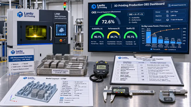
Consider one metal LPBF machine over a seven-day reporting period. Calendar time is 10,080 minutes. After deducting 240 minutes of planned maintenance and 1,440 minutes of breaks, loading time is 8,400 minutes. Downtime losses are: powder change and chamber cleaning, 360 minutes; protective window and optical path, 180 minutes; recoater and filters, 150 minutes; waiting for powder certificates, 240 minutes; waiting for inspection reports, 180 minutes; and failures, 210 minutes. The total is 1,320 minutes, leaving 7,080 minutes of operating time. Availability = 7,080/8,400 = 84.3%. After recalculation from the parameter set, the theoretical cycle time indicates that 118 equivalent parts should have been completed during operating time. Second-level event logs show that micro-stoppages and speed reductions caused an equivalent loss of 960 minutes. The speed rate is approximately 86.4%, resulting in a performance figure of approximately 72.8%. Of 96 input parts, four were scrapped due to CTQ deviations; one build with six parts was rejected in full because its witness coupon failed; and two repaired parts were subsequently released. Final conforming output was 88 parts, so Quality Rate = 88/96 = 91.7%. OEE = 84.3% × 86.4% × 91.7% ≈ 66.8%. Ranking losses by minutes in a Pareto chart gives: material and inspection waiting, 420 minutes; micro-stoppages, 960 equivalent minutes; powder change and chamber cleaning, 360 minutes; and six parts affected by full-build scrap. The first two account for nearly 60% of losses. The real bottleneck is not machine failure, but upstream certificate/report readiness and process-parameter stability. If attention remains fixed on the 210 minutes of breakdown time, no amount of equipment investment will materially increase OEE. This conclusion becomes visible only when all six big losses are converted to a common unit.

6. Data Chain and Anti-Gaming Controls: Align Four Sources and Prohibit Manual Entry

OEE is most at risk of becoming a manually completed month-end spreadsheet. The minimum credible data chain requires line-by-line alignment of four sources: second-level equipment event logs, including build ID, layer number, oxygen level, power fluctuations, and micro-stoppages; work-order reporting records, including start/completion/interruption timestamps and loss codes; parameter-set versions and hashes, proving which scan strategy was used for theoretical cycle-time calculation; and inspection records for CTQs and witness-coupon release, proving the numerator of the quality rate. All four sources must use the same clock source, with build ID as the primary key. Backfilling entries such as “estimated downtime: two hours” is prohibited. Where a supplemental entry is unavoidable, it must retain audit-trail fields: person entering the record, original value, reason, and reviewer. The metric should also interface with adjacent engineering systems: loading time should share the same machine calendar used for finite-capacity scheduling; component-level energy consumption within performance can be cross-checked against submetering data, since purge-and-rescan cycles necessarily create abnormal kWh usage; and full-build rejection for quality must be written back to the inspection lot and witness-coupon evidence chain. OEE should not be used to assess individual shifts or teams, otherwise personnel will tend to move failed builds into “planned downtime,” immediately distorting the metric. It should be used only to identify the loss structure and verify whether improvement actions are effective.

Conclusion: Anchor Efficiency Metrics to an Auditable Minute-by-Minute Chain

Implementation should follow five steps. First, freeze the Statistical Definition Card, including the loading-time definition, cross-shift allocation, multi-part build allocation, repair-counting rules, and the rule that definitions cannot change within a quarter. Second, create a loss-code table for additive-specific downtime and micro-stoppages, with standard times and trigger thresholds. Third, recalculate theoretical cycle time from parameter sets rather than using supplier nominal values. Fourth, link acceptance decisions to CTQ reinspection and witness coupons; full-build impact must enter the denominator. Fifth, align the four logs by build ID, issue a monthly loss Pareto chart, and focus improvement only on the top two losses. Five common failure modes are: using calendar time as loading time; recording material waiting as normal equipment time; guessing theoretical cycle time; counting visually acceptable parts as conforming; and manually backfilling records at month-end. Avoid these five errors, and OEE becomes engineering data that a third party can audit minute by minute rather than a slogan—truly supporting capacity commitments from blueprint to delivery.